Planar Data Classification With One Hidden Layer

15/9/2025
3-minute read

For Week 3 of the Deep Learning Specialization, we move beyond logistic regression and build our first neural network — one with a single hidden layer. The task is to classify a toy flower-shaped dataset, which logistic regression cannot handle well.

The Problem

The dataset looks like a set of flower petals spread around the origin. Logistic regression struggles here because the decision boundary is non-linear.

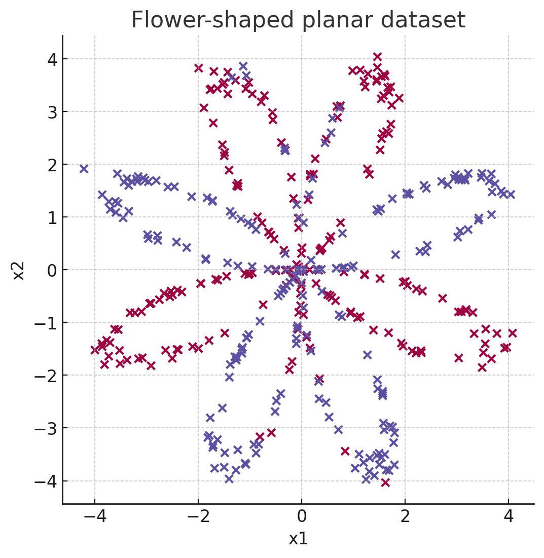
Flower-shaped planar dataset used in Week 3

Neural Network Architecture

We design a 2-layer neural network:

Input layer: 2 features (x₁, x₂)
Hidden layer: 4 neurons with tanh activation
Output layer: 1 neuron with sigmoid activation (binary classification)

Forward Propagation

Forward propagation computes the activations layer by layer. + Mathematically:

$$ Z^{[1]} = W^{[1]} X + b^{[1]} \newline A^{[1]} = \tanh(Z^{[1]}) \newline Z^{[2]} = W^{[2]} A^{[1]} + b^{[2]} \newline \hat{Y} = A^{[2]} = \sigma(Z^{[2]}) $$

In code, forward pass looks like:

def forward_propagation(X, parameters):
    W1, b1 = parameters["W1"], parameters["b1"]
    W2, b2 = parameters["W2"], parameters["b2"]

    Z1 = np.dot(W1, X) + b1
    A1 = np.tanh(Z1)
    Z2 = np.dot(W2, A1) + b2
    A2 = sigmoid(Z2)

    cache = {"Z1": Z1, "A1": A1, "Z2": Z2, "A2": A2}
    return A2, cache

Cost Function – Cross-Entropy Loss

We use the standard cross-entropy loss:

$$ J = -\frac{1}{m} \sum_{i=1}^{m} \Big[ y^{(i)} \log(\hat{y}^{(i)}) + (1-y^{(i)}) \log(1-\hat{y}^{(i)}) \Big] $$

This penalizes confident wrong predictions heavily, encouraging the network to output probabilities close to the true labels.

def compute_cost(A2, Y):
    m = Y.shape[1]  # number of examples
    logprobs = (np.multiply(np.log(A2),Y)) + (np.multiply((1 - Y), np.log(1 - A2)))
    cost = -(1/m) * np.sum(logprobs)
    return np.squeeze(cost)  # ensure it's a scalar

Backward Propagation

The key to training is computing gradients:

$$ dZ^{[2]} = A^{[2]} - Y \newline dW^{[2]} = \frac{1}{m} dZ^{[2]} A^{[1]T} \newline db^{[2]} = \frac{1}{m} \sum dZ^{[2]} $$

For the hidden layer:

$$ dZ^{[1]} = (W^{[2]T} dZ^{[2]}) \odot (1 - A^{[1]^2}) \newline dW^{[1]} = \frac{1}{m} dZ^{[1]} X^T \newline db^{[1]} = \frac{1}{m} \sum dZ^{[1]} $$

def backward_propagation(parameters, cache, X, Y):
    m = X.shape[1]

    W2 = parameters["W2"]

    A1, A2 = cache["A1"], cache["A2"]

    dZ2 = A2 - Y
    dW2 = (1/m) * np.dot(dZ2, A1.T)
    db2 = (1/m) * np.sum(dZ2, axis=1, keepdims=True)

    dZ1 = np.dot(W2.T, dZ2) * (1 - np.power(A1, 2))
    dW1 = (1/m) * np.dot(dZ1, X.T)
    db1 = (1/m) * np.sum(dZ1, axis=1, keepdims=True)

    grads = {"dW1": dW1, "db1": db1, "dW2": dW2, "db2": db2}
    return grads

Parameter Update

We update parameters using gradient descent:

$$ W^{[l]} := W^{[l]} - \alpha , dW^{[l]} \newline b^{[l]} := b^{[l]} - \alpha , db^{[l]} $$

where $\alpha$ is the learning rate.

def update_parameters(parameters, grads, learning_rate=1.2):
    parameters["W1"] -= learning_rate * grads["dW1"]
    parameters["b1"] -= learning_rate * grads["db1"]
    parameters["W2"] -= learning_rate * grads["dW2"]
    parameters["b2"] -= learning_rate * grads["db2"]
    return parameters

Putting It All Together

Now that we have forward propagation, cost computation, backward propagation, and parameter updates, we can combine them into one training loop.

def nn_model(X, Y, n_h, num_iterations=10000, learning_rate=1.2, print_cost=False):
    np.random.seed(3)
    n_x = X.shape[0]
    n_y = Y.shape[0]

    # Initialize parameters
    parameters = initialize_parameters(n_x, n_h, n_y)

    for i in range(num_iterations):
        # Forward propagation
        A2, cache = forward_propagation(X, parameters)

        # Compute cost
        cost = compute_cost(A2, Y)

        # Backward propagation
        grads = backward_propagation(parameters, cache, X, Y)

        # Update parameters
        parameters = update_parameters(parameters, grads, learning_rate)

        if print_cost and i % 1000 == 0:
            print(f"Iteration {i}, cost: {cost}")

    return parameters

Results

Logistic regression achieves only ~47% accuracy on this dataset.
Our 2-layer neural network achieves ~90%+ accuracy.
The decision boundary is non-linear and adapts to the flower shape.

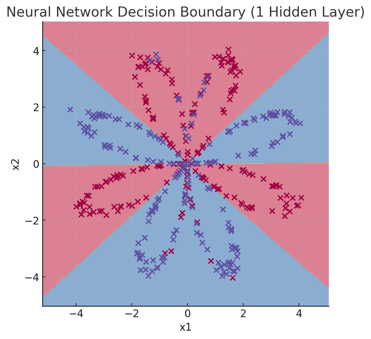
Decision boundary learned by the hidden-layer neural network

Key Takeaways

Adding a hidden layer lets us capture non-linear patterns.
tanh works well for hidden layers, while sigmoid is used for binary output.
Forward + backward propagation form the core training loop.
Even a shallow network can vastly outperform logistic regression on complex data.

Posts in this series

coursera deeplearning neuralnetworks