Building Deep Neural Networks
In Week 2, we trained a logistic regression classifier for the cat vs. non-cat dataset. It reached about 70% test accuracy, but logistic regression is fundamentally limited: it can only draw one linear boundary.
This week, we built deep neural networks from scratch and apply them to the same dataset.
- First: 2-layer network
- Then: 4-layer network
Both outperformed logistic regression - and the deeper model gave the best results.
Neural Network Architecture
- 2-Layer Model
INPUT → LINEAR → RELU → LINEAR → SIGMOID → OUTPUT - L-Layer Model (generalized)
[LINEAR → RELU] × (L-1) → LINEAR → SIGMOID
Forward Propagation
For each layer \( l \):
$$ Z^{[l]} = W^{[l]} A^{[l-1]} + b^{[l]} \newline A^{[l]} = g(Z^{[l]}) $$
where \( g \) is ReLU for hidden layers, and sigmoid for the final output.
Cost Function
We used cross-entropy loss:
$$ J = -\frac{1}{m} \sum_{i=1}^m \Big[ y^{(i)} \log \hat{y}^{(i)} + (1 - y^{(i)}) \log (1 - \hat{y}^{(i)}) \Big] $$
Backward Propagation
Gradients for layer \( l \):
$$ dZ^{[l]} = dA^{[l]} \odot g’(Z^{[l]}) $$ $$ dW^{[l]} = \frac{1}{m} dZ^{[l]} (A^{[l-1]})^T $$ $$ db^{[l]} = \frac{1}{m} \sum dZ^{[l]} $$
Update step:
$$ W^{[l]} = W^{[l]} - \alpha dW^{[l]} $$ $$ b^{[l]} = b^{[l]} - \alpha db^{[l]} $$
Dataset Setup
We used the cat vs non-cat dataset (209 training, 50 test). Each 64×64 RGB image is flattened into a vector of size 12,288.
train_x_orig, train_y, test_x_orig, test_y, classes = load_data()

# Flatten and normalize
train_x = train_x_orig.reshape(train_x_orig.shape[0], -1).T / 255.
test_x = test_x_orig.reshape(test_x_orig.shape[0], -1).T / 255.

print("train_x shape:", train_x.shape)
print("test_x shape:", test_x.shape)
Output:
train_x shape: (12288, 209)
test_x shape: (12288, 50)
Two-Layer Model
n_x = 12288 # input size
n_h = 7     # hidden layer size
n_y = 1     # output size
layers_dims = (n_x, n_h, n_y)

parameters, costs = two_layer_model(train_x, train_y, layers_dims,
                                    num_iterations=2500, learning_rate=0.0075,
                                    print_cost=True)
plot_costs(costs)
Training Curve:
Results:
- Training accuracy: ~100%
- Test accuracy: 72%
Four-Layer Model
layers_dims = [12288, 20, 7, 5, 1]

parameters, costs = L_layer_model(train_x, train_y, layers_dims,
                                  num_iterations=2500, learning_rate=0.0075,
                                  print_cost=True)
plot_costs(costs)
Training Curve:
Results:
- Training accuracy: 98.5%
- Test accuracy: 80%
Comparison
To see how depth helps, here’s both curves side by side:
- Logistic Regression (Week 2): 70% test accuracy
- 2-layer NN: 72% test accuracy
- 4-layer NN: 80% test accuracy
Clearly, deeper networks generalize better.
Error Analysis
We printed mislabeled images:
pred_test = predict(test_x, test_y, parameters)  # parameters from 4-layer model
print_mislabeled_images(classes, test_x, test_y, pred_test)
Common errors:
- Cats in unusual poses
- Background colors similar to the cat
- Low lighting or overexposure
- Cats that are too zoomed in or very small
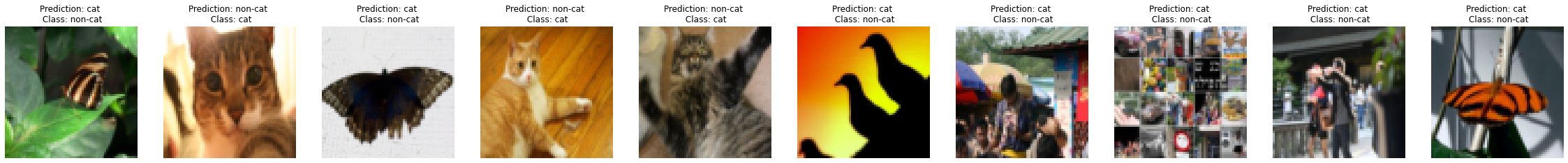
Mislabeled Images
Key Takeaways
- Logistic regression = single-layer neural network.
- Deep networks stack linear + non-linear transformations to learn richer features.
- Vectorized implementation makes training feasible.
- Deeper models improve accuracy, but data and regularization matter.
This marks the end of Course 1 - next comes hyperparameter tuning, optimization algorithms, and regularization in Course 2.